Tutorial: groups in the scikit-learn digits dataset, part 1¶

This tutorial runs Starfold once on the scikit-learn digits dataset and reads the first half of the result: the run, the flags, the map and the chosen settings. The dataset is a copy of the UCI handwritten digits test set: 1,797 images of 8 by 8 pixels, one per row, with 64 pixel columns. It follows the notebook notebooks/01_digits.ipynb, so you can run the cells there while you read. Part 2 (Tutorial: groups in the scikit-learn digits dataset, part 2) reads support, recurrence, the group count and the comparison with the true digits, and saves the result.

Goal¶

By the end of this part you have a finished run, you know whether it raised a warning, and you have seen a map of the groups and the settings the search chose.

Before you start¶

Python 3.11 or 3.12 and a clone of the repository (the notebooks need the clone). The full install page is Install Starfold. From a terminal:
```
git clone https://github.com/AndreasWNeitzel/starfold && cd starfold
uv sync --extra bench
```
Add --extra gpu-cu13 or --extra gpu-cu12 to uv sync if you have an NVIDIA GPU and want cuML (NVIDIA’s GPU versions of UMAP and HDBSCAN). Without it Starfold runs on the CPU.
Time: the recorded run took 93.9 s on a laptop RTX 3060 with cuML (search 77.4 s, refits 7.2 s, 314 fits, 1,422 MB peak host memory). The CPU time is not measured, so plan for longer.
The numbers below come from that recorded run with random_state=0. A different engine or machine can change the last digits.

The table is 1,797 row entries, one per image, and 64 column entries, one per pixel of an 8 by 8 picture. Each pixel value runs from 0 (dark) to 16 (bright).

Step 1: load the table¶

Load the images. Keep the true digits in y. Starfold never reads y.

from sklearn.datasets import load_digits

X, y = load_digits(return_X_y=True)
print(f"{X.shape[0]} images, {X.shape[1]} pixel columns, values {X.min():.0f} to {X.max():.0f}")
print(f"true digits, kept aside: {len(set(y))} classes")

The two lines print:

1797 images, 64 pixel columns, values 0 to 16
true digits, kept aside: 10 classes

The table has no missing values and needs no cleaning. If yours has missing or infinite values, Starfold drops those rows and raises a flag (you meet flags in step 3).

Step 2: call `recover`¶

One call does the whole procedure. Starfold searches for a setting with Optuna, fits the chosen setting once on all rows, refits it 32 times on random 80 percent subsets, checks the result and raises flags.

import starfold

result = starfold.recover(X, random_state=0)
print(f"groups in the fit on all rows: {result.n_groups}")

The run takes about a minute and a half on the recorded GPU, then prints:

groups in the fit on all rows: 10

A refit is one more fit of the chosen setting on a random subset with a new seed. The fit on all rows gives result.labels: one integer per kept row, the group number or -1 for noise. Group numbers are names, not ranks.

Ten is the number of groups of one fit and not yet a finding. Steps 7 and 8 show how much it moves.

To see what ran, print the provenance:

prov = result.provenance
print(f"engine: asked for {prov['engine_requested']}, used {prov['engine_resolved']}")
print(f"rows kept: {prov['n_kept_rows']} of {prov['n_input_rows']}, columns: {prov['n_features']}")
print("fits per stage:", prov["stage_fits"], "total", prov["total_fits"])

The recorded run prints:

engine: asked for auto, used cuml
rows kept: 1797 of 1797, columns: 64
fits per stage: {'search': 280, 'reference': 2, 'worlds': 32, 'null': 0} total 314

All 1,797 rows were kept, so every row is in the result. Always check that the engine you asked for is the engine used.

Step 3: read the flags¶

A flag is a short name for one weakness or event in a run. Read the flags before any number.

from starfold.result import FLAG_VOCABULARY

print(f"{len(result.flags)} of {len(FLAG_VOCABULARY)} flags raised")
for flag in result.flags:
    print(f"- {flag}")

Four flags are raised:

4 of 17 flags raised
- search_budget_exhausted
- count_unstable
- consensus_disagrees
- null_not_run

Read them one at a time.

search_budget_exhausted: all 48 trials ran. This says how the search ended. A larger n_trials might find a better setting.
count_unstable: fewer than half of the refits found 10 groups. The count is not reproducible. Step 8 shows by how much.
consensus_disagrees: a second check gave a different grouping. The check counts, for every pair of rows, how often the refits put the pair together (co-association), and cuts the rows into groups from those counts. The cut matched your labels with a score of 0.135, below the 0.5 threshold. This is not an error. Read the contrast before you conclude anything.
null_not_run: the calibration test did not run, so there is no p-value. Expected, because the test is off by default.

For a pair of rows, co-association is the share of the refits that assigned both rows and put them in the same group. The contrast is the mean co-association of pairs inside your groups minus the mean for pairs in different groups. The recorded values are:

within-group co-association:  0.820
between-group co-association: 0.068
contrast:                     0.751
agreement of the cut with labels (ARI times coverage): 0.135

The contrast of 0.751 says pairs inside a group were grouped together far more often than pairs in different groups. The consensus agreement (the cut against your labels, adjusted Rand index times coverage) is 0.135: the cut found 3 groups (the notebook prints groups in the cut: 3) where your labels have 10. Both are true at once, so consensus_disagrees is a prompt to look, not a verdict. The full list of flags is in Flags.

Step 4: draw the map¶

The groups were found in a map of 4 coordinates. A screen has two, so the notebook cell “A picture of the groups” makes one more UMAP fit in 2 coordinates for display only. It uses the deployed n_neighbors and min_dist and draws three panels. You can run that cell, or draw a plain version of the middle panel yourself. In the plain version noise gets a colour and there is no opacity, so it will not match the figure exactly:

import matplotlib.pyplot as plt
import umap
from sklearn.preprocessing import StandardScaler

p = result.deployed_params
layout = umap.UMAP(
    n_neighbors=p.n_neighbors, min_dist=p.min_dist, n_components=2, random_state=0
).fit_transform(StandardScaler().fit_transform(X[result.kept_rows]))
plt.scatter(*layout.T, c=result.labels, s=3, cmap="tab10")
plt.xlabel("display axis 1")
plt.ylabel("display axis 2")
plt.show()

The notebook figure looks like this.

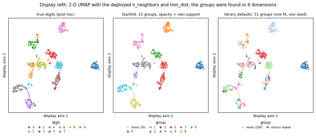
Three maps of the digits: the true digits, Starfold's 10 groups with opacity set by own support, and 51 groups from the library defaults.

Every dot is one image. The axes are display axes with no units and no ticks: only which dots sit near which dots means anything, and the gaps between islands should not be over-read. The left panel colours each dot by its true digit (post hoc, meaning “after the fact”). The middle panel colours each dot by Starfold’s group, and a faint dot has low own support (the share of refits that kept the row with its group). Grey dots are noise, 30 of them. The right panel shows one fit of the library defaults, with 51 groups.

A good picture has compact islands with mostly solid dots, and few grey dots between them. The middle panel is close to that. A bad picture has islands cut into many small clumps of different colours. The right panel shows it: one fit of the defaults splits several digits into pieces and calls 189 rows noise.

Treat the map as a first look. The numbers in the next steps decide what to trust.

Step 5: read the settings the search chose¶

A setting is one complete choice of six values: n_neighbors, min_dist and n_components for UMAP, and min_cluster_size, min_samples and selection_method for HDBSCAN. Print the chosen setting, the one that made labels, and the library defaults:

columns = {
    "chosen": result.params,
    "deployed": result.deployed_params,
    "defaults": result.default_params,
}
print(f"{'setting':<20}" + "".join(f"{name:>12}" for name in columns))
for name in result.params.to_dict():
    row = "".join(f"{p.to_dict()[name]:>12.3f}" if isinstance(p.to_dict()[name], float)
                  else f"{p.to_dict()[name]:>12}" for p in columns.values())
    print(f"{name:<20}{row}")

The table it prints:

setting                   chosen    deployed    defaults
n_neighbors                   13          13          15
min_dist                   0.262       0.262       0.100
n_components                   4           4           2
min_cluster_size              11          14           5
min_samples                    9          11           5
selection_method             eom         eom         eom

The chosen column is the setting as searched, on 80 percent subsets. The deployed column is the setting fitted on all rows: min_cluster_size and min_samples count rows, so they are scaled up by the ratio of the row counts.

Next, the search summary and the candidates that Starfold scored again on fresh subsets (the fresh re-score):

s = result.search
print(f"trials run: {len(s.trials)} of 48; stop reason: {s.stop_reason}")
print(f"fresh gap: chosen {s.gap_selected:.3f}, defaults {s.gap_default:.3f}")
print(f"beats the defaults under the objective: {s.beats_default_under_objective}")

The recorded run prints:

trials run: 48 of 48; stop reason: budget
fresh gap: chosen 0.661, defaults 0.565
beats the defaults under the objective: True

Every trial got a score, a number built from prediction agreement, coverage and modularity. Starfold then scored the same setting on a structureless copy of the table and subtracted it. The difference is the gap, and the search tries to make the gap large. The score never reads the number of groups. The figure plots the trials.

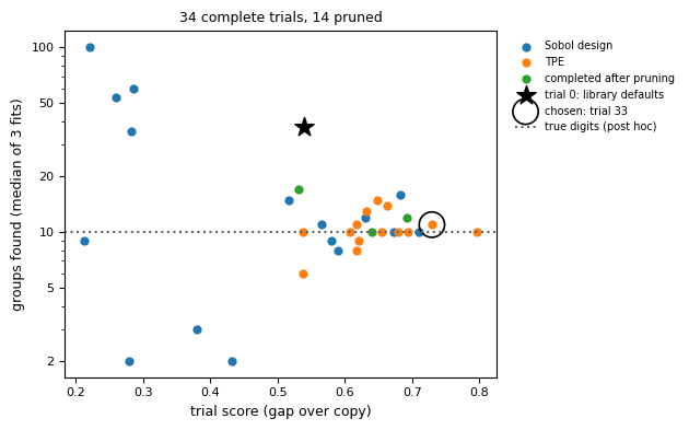
Each dot is one finished trial. The horizontal axis is the gap (the figure labels it “trial score (gap over copy)”). The vertical axis is the number of groups its fits found, on a logarithmic scale. Blue dots are the Sobol design, orange dots are TPE proposals, green dots are pruned trials finished at the end. The star is the library defaults, between 30 and 40 groups, at a gap near 0.54. The ring is the chosen trial 33. The dotted line at 10 is the true number of digits (post hoc).

Look at the shape of the cloud. Trials with a low gap (left) scatter from 2 to 100 groups. Trials with a high gap (right) gather between about 8 and 16. A good picture of a search has high gaps that agree on a count. A bad picture has high gaps at widely different counts, which would mean the table supports many readings.

The chosen setting beat the defaults on the fresh gap, 0.661 against 0.565. The fresh re-score reduces the winner’s curse (the best of many noisy scores is partly luck) but does not remove it. The six paired differences between them were [0.087, 0.032, 0.075, 0.004, 0.045, -0.016], and one is negative. The flag default_within_noise was not raised, but its noise estimate treats six overlapping pair differences as independent, so read it as a coarse screen and the margin as small. See Score, Gap and Default comparison.

What you learned¶

A run ends in flags first. Read them before any number.
Four of 17 flags were raised. None says the search found nothing, and consensus_disagrees is read together with the contrast.
The group count of one fit (10) is not yet a finding.
The search chose a setting that beat the defaults on the fresh gap, by a small margin.

Next page¶

Go on to Tutorial: groups in the scikit-learn digits dataset, part 2: support, recurrence, the group count, the comparison with the true digits, and saving the result.