Copies and gaps
This page explains why a good score alone is not evidence of groups, what a structureless copy is, and why Starfold’s search maximises the gap over a copy.
A score alone proves nothing
UMAP, HDBSCAN and Optuna together can find groups in almost any table, including one with none. Imagine a smooth round cloud of points. Cut it into compact pieces and the pieces come back when you refit, look tidy, and follow the neighbour links. A search that tries 48 settings finds the setting that does this best. The score is high, and no group is there.
So Starfold never reads a score on its own. It asks how much higher the score is on your table than on copies that keep each column but lose the structure across columns.
The score and the gap are different numbers. The score is one number for one setting on your table. The gap is that score minus the score of the same setting on a copy. By default the search maximises the gap.
What a structureless copy is
A structureless copy is your table with every value kept and the pairing of values across columns redrawn. It invents nothing. Each column of the copy holds exactly the values that column holds in your table. Only the choice of which row holds which value changes.
The marginal of a column is its values on their own, ignoring the other columns, as a histogram of that one column shows. Starfold has two families of copy:
gaussian_copula(the default). It keeps every column’s values and roughly the overall tilt between columns, and removes clumps that show only when columns are combined. The steps are below.independent_marginals. It shuffles each column on its own. The copy keeps every histogram and loses all trends.
How a gaussian_copula copy is built
The next steps use a toy table of 5 rows and 2 columns, A and B. The numbers are made up to show the mechanics. They are not from a run.
Row |
A |
B |
|---|---|---|
1 |
2 |
30 |
2 |
9 |
80 |
3 |
4 |
10 |
4 |
7 |
60 |
5 |
5 |
50 |
Measure the tilt. Starfold replaces each value by its rank inside its column, and measures how strongly A and B move together on those ranks. Ranks ignore the shape of each histogram, so only the relationship between columns is left.
Draw random points with that tilt. It draws 5 new random points from a smooth cloud with about the same tilt. Say the first coordinates of the draw are -0.3, 1.2, 0.1, -1.1 and 0.6 for the rows 1 to 5.
Put your real values back in that order. The smallest drawn coordinate goes to the smallest real value of A, the next to the next, and so on. Row 4 has the smallest draw, so it receives 2. Rows 1, 3, 5 and 2 receive 4, 5, 7 and 9. The same happens for column B.
Read the copy. If the draw for B gives row 4 the smallest, then rows 3, 1, 2 and 5 after it, the copy is:
Row |
A |
B |
|---|---|---|
1 |
4 |
50 |
2 |
9 |
60 |
3 |
5 |
30 |
4 |
2 |
10 |
5 |
7 |
80 |
Column A still holds 2, 4, 5, 7 and 9, and column B still holds 10, 30, 50, 60 and 80. Only the pairing of values across columns changed. The tilt stays because the draw had it, and the clumps go because the draw was one smooth cloud. In the code the correlation is the Ledoit-Wolf shrinkage estimate of the normal scores of each column. The copy has one Gaussian dependence structure (elliptical in rank space, which is the Gaussian copula) with every column’s observed marginal. In data space it can still be skewed or two-peaked, because the marginals are kept exactly.
The copy on real data
The next figure uses the APOGEE DR19 example table from the second tutorial, which holds 9,242 stars. [Fe/H] is the iron abundance of a star and [Mg/Fe] its magnesium abundance relative to iron, both in dex (a logarithmic unit).
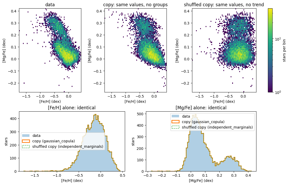
Look at the top row first. The data (left) show a tilted band with a second, higher band. The copy in the middle has about the same tilt and the same overall spread, but no second band. The shuffled copy (right) has no tilt. Then look at the bottom row. The three histograms coincide, because a copy only reorders each column. On this table the recorded Spearman correlation (rank correlation) between the two columns is -0.67 for the data, -0.61 for the gaussian_copula copy and +0.00 for the shuffled copy.
A copy keeps what shows in one column alone, such as two peaks, and removes structure that shows only when columns are combined. A test against gaussian_copula copies therefore asks for more than a trend between columns. The table must score higher than tables that have that trend and nothing else.
The gap
The gap of a setting is its score on your table minus its score on a copy, fitted with the same setting. A setting that scores as well on structureless data gains nothing from it, so its gap is near zero. During the search, each trial’s gap uses one copy that stays fixed. The fresh re-score at the end averages over three new copies.
The search maximises the gap, not the score. This steers it away from settings that find tidy pieces in any cloud, and toward settings that find something your table has and its copy lacks. The idea follows the gap statistic of Tibshirani, Walther and Hastie (2001, doi:10.1111/1467-9868.00293). The Gap page says how to read a value. With Config(gap_family=None) or Config(n_null_rescore=0) no copy is fitted, and the search ranks settings by the score itself.
A high gap does not prove the groups are real. It says the table scores above copies that keep each column’s values and one Gaussian dependence between columns.
The calibration test
The optional calibration test asks the same question of the whole procedure. By default it replays trials 0 to 16 (the library defaults and the 16-trial Sobol design) on up to 19 copies. It compares the largest search gap among those 17 trials on each copy with the same quantity on your table. The option null_procedure="full_search" replays the whole search instead.
The p-value is the share of copies whose statistic is at least as high as the table’s, counting the table as one more draw. If the table is a draw from the declared family of copies, a p-value at or below 0.05 comes up at most about 5 percent of the time. Ties and the stopping rule keep p from being spread exactly evenly.
The recorded results in bench/results used 19 gaussian_copula copies and an alpha of 0.05:
The scikit-learn digits dataset: the table’s statistic was 0.710, the search gap of trial 7. No copy reached it, so p = 0.05. Structure is supported against this family.
The APOGEE DR19 example table: the table’s statistic was 0.362 and one copy scored higher, so p = 0.10. The test gives no support for structure in the table as a whole, which is different from showing that the table has no groups.
The p-value holds only for the declared family of copies and the procedure that was simulated. It is not the probability that the groups are real. With 19 copies the smallest possible p is 1 in 20, which is 0.05. So p = 0.05 is the best result this test can give, and it does not separate a clear win from a narrow one. The 0.05 floor and the rule that the test stops after three copies reach the table hold at the default 19 copies only. The Calibration p-value page has the details.
Learn more
Gap: how to read a gap value.
scikit-learn clustering guide: clustering metrics side by side, including the adjusted Rand index. Starfold uses that index inside its prediction agreement, one of the three parts of the score.
HDBSCAN comparison of clustering algorithms: where other algorithms find groups that are not there.