Plot your result

This guide points at the plotting cells of the notebooks, names the attribute each plot reads, and shows how to read two of them. The notebooks hold the full code, so this page does not repeat it.

Prerequisites

• A result from starfold.recover, or one loaded with Save a result and load it back.

• A clone of the repository, with uv sync --extra bench, so that you can open notebooks/01_digits.ipynb.

• matplotlib. Every plot below needs only that and the result. Plots marked post hoc also need known labels (Check a result against known labels).

Steps

1. Open notebooks/01_digits.ipynb. Its first cell finds the repository root and its parameters cell sets RANDOM_STATE, ENGINE, N_JOBS and FIGURES. Set FIGURES to a folder to save each figure as it is drawn.

2. Replace the data cell and the recover cell with your own table and result. Every plotting cell after them reads only from result.

3. Run the plotting cells in the order below. Each row names the heading of the cell in notebooks/01_digits.ipynb and what it reads.

   Heading of the cell	Reads	Shows
   A picture of the groups	result.labels, result.worlds.own_support, result.default_labels	the rows on a 2-D map, in three panels: known classes (post hoc), Starfold, library defaults
   Settings against groups	result.search.trials, each trial’s score, fit_counts and phase	the score of every complete trial against the groups it found
   Support per row	result.worlds.own_support, result.worlds.unresolved	how reliably each grouped row comes back
   Recurrence per group	result.worlds.group_recurrence and group_recurrence_band	how often each group comes back, and the group sizes
   How many groups	result.worlds.count_values and count_interval	the groups found in each refit
   The co-association check	result.consensus	within-group, between-group and contrast values

   The notebook draws the map in 2-D by fitting UMAP again with the chosen n_neighbors and min_dist. If the chosen map has more than two coordinates, the picture is a separate 2-D display map and not the space in which the groups were found.

4. Save the figures as PDF if they are for a paper. The notebook writes PNG at 150 dpi for the manual. Change the extension and the savefig call in save_figure.

5. For the structureless copies and the calibration histograms, use notebooks/03_calibration.ipynb (starfold.generate_null(x, family, seed=0) makes a copy). For physical units of the groups, use the cell “The groups in physical units” in notebooks/02_apogee.ipynb, which reads result.worlds.property_median and property_band.

Reading two plots

Groups found in each refit

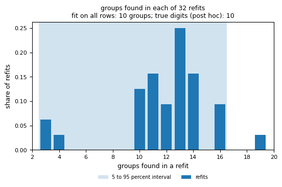
The bars show how many refits found each group count. Most of the mass lies between 10 and 14 groups, and a few refits found 3, 4 or 19. The shaded band is the stability interval, 3 to 16. The fit on all rows has 10 groups, and only about one refit in eight (4 of 32) found exactly 10. Quote the interval and not the single count. This run raises count_unstable, which means fewer than half the refits found the same count as the fit on all rows. The count is not an estimate of how many populations exist (count interval).

Recurrence of each group

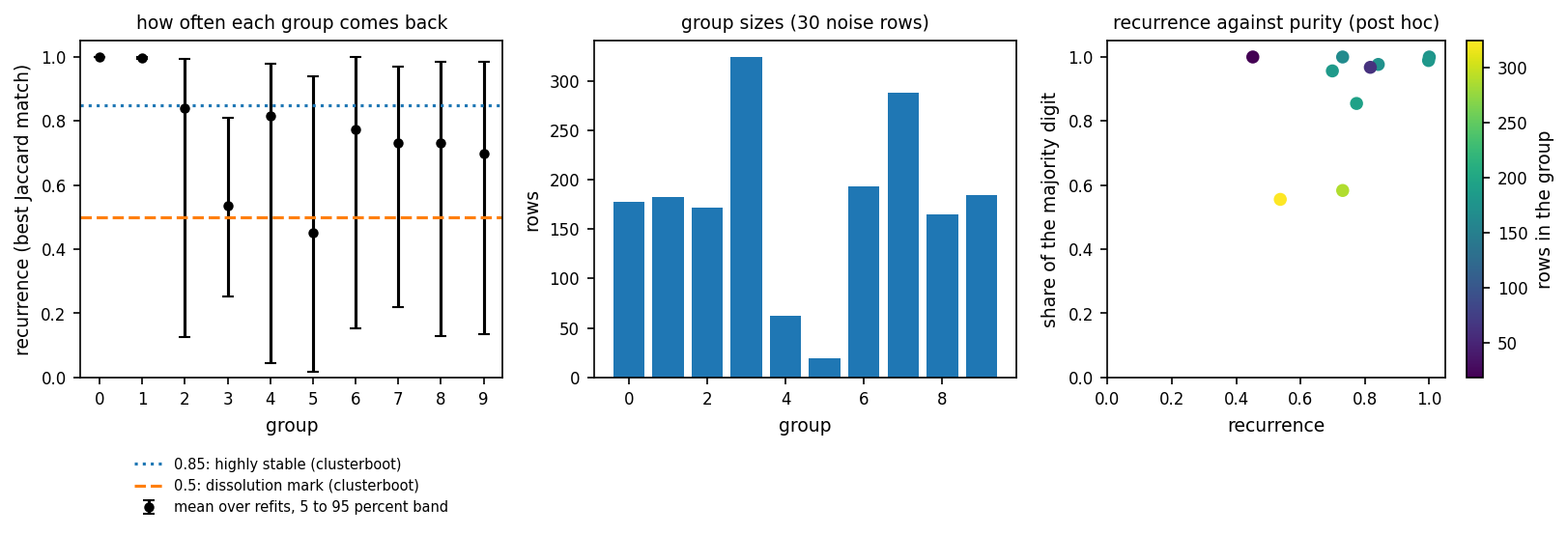
The left panel shows one dot per group, with a band over refits. Groups 0 and 1 sit at 1.00 with no visible band, so they come back in almost every refit. Group 5, the smallest (19 rows), has the lowest value, 0.45 (band 0.02 to 0.94), and group 3 has 0.54 (0.25 to 0.81). The other six lie between 0.70 and 0.84, with wide bands whose lower ends run from 0.05 to 0.22. The dotted line at 0.85 and the dashed line at 0.5 are the clusterboot marks (R package fpc) for a highly stable mean and for a cluster that dissolved in one resample. Starfold quotes them and never uses them to drop a group. Describe groups 0 and 1 as reproducible and treat the wide-band groups as uncertain. Read the right panel (post hoc) before you say anything about what a group is. Recurrence is how often a group comes back across refits, not a probability. See Group recurrence.

Expected result

You get five figures and one printed check for your result. Read each figure axis by axis and say what it lets you report, as in the two readings above. The Digits notebook reproduces the figures of this manual from the recorded run in notebooks/runs/digits. The saved runs in notebooks/runs/ ship with the repository, and notebooks 01 and 02 write them.

Variations

• Replot without refitting. Load the saved result with starfold.load("notebooks/runs/digits") and run only the plotting cells.

• Your own figure. Every array the notebooks plot is an attribute listed in Saved result files.

Related pages

• Tutorials

• Support and own support

• Count interval

• Save a result and load it back