Tutorial: two groups in the APOGEE DR19 example table, part 2¶

This page checks the two APOGEE groups with the co-association check and the calibration test, then writes down what the run supports. It continues Tutorial: two groups in the APOGEE DR19 example table, part 1 and follows the second half of the notebook notebooks/02_apogee.ipynb.

Goal¶

You finish with two more pieces of evidence for how far to trust the two groups (co-association and a calibration test) and a paragraph you can put in a paper.

Before you start¶

Finish Tutorial: two groups in the APOGEE DR19 example table, part 1. Keep the same Python session, because steps 8 to 10 use result, x, names and starfold from there.
If you start a new session, load the recorded run from the clone instead. The saved runs in notebooks/runs/ ship with the repository, and notebooks 01 and 02 write them. Run Python from the repository root:
```
import starfold
from bench.datasets import example_table

x, names = example_table()
result = starfold.load("notebooks/runs/apogee")
```
Step 10 runs a command that takes about 36 minutes on the recorded hardware, or you can read the recorded result without running it.
The numbers below come from the recorded run with random_state=0. A different engine or machine can change the last digits.

Step 8: run the co-association check¶

Group numbers are arbitrary: one refit’s group 0 may be another’s group 1. The check needs no matching, because it asks only whether two stars share a group. For a pair of stars, the co-association is the share of refits that assigned both and put them in the same group. Pairs in the same group should sit near 1 and pairs in different groups near 0. The contrast is the mean over same-group pairs minus the mean over different-group pairs.

c = result.consensus
print(f"{c.n_rows:,} stars ({'seeded subset' if c.subsampled else 'all'}): "
      f"within {c.within_association:.3f}, between {c.between_association:.3f}, "
      f"contrast {c.contrast:.3f}, cut agreement {c.agreement:.3f}")

The recorded run prints:

4,096 stars (seeded subset): within 0.979, between 0.003, contrast 0.976, cut agreement 0.000

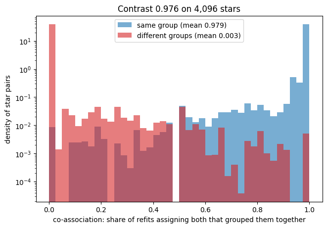
Histogram of co-association for star pairs in the same group (blue) and in different groups (red), with a logarithmic vertical axis.

The horizontal axis is the co-association of a pair, from 0 to 1. The vertical axis is the density of pairs on a logarithmic scale, so rare values show. The blue histogram (same group) has a tall spike at 1 and a mean of 0.979. The red histogram (different groups) has a tall spike at 0 and a mean of 0.003. Between 0.1 and 0.9 both histograms sit between about 0.0001 and 0.06, against about 40 at the spikes, so few pairs are undecided.

A good picture has the two spikes at opposite ends. A bad picture has both histograms centred in the middle, where refits disagree about which stars belong together.

In the recorded run the regrouping failed. The check also regroups the stars: it runs HDBSCAN on the co-association turned into a distance, and compares that cut with the partition. The consensus agreement (printed as “cut agreement”: the cut against the partition, adjusted Rand index times coverage) is 0.000. The cut assigned every one of the 4,096 stars to no group. That is why consensus_disagrees is raised. The cause of the all-noise cut was not diagnosed. The code notes that rows at the floor distance can let the cut merge neighbouring groups.

The failed cut does not mean the groups are absent. The contrast of 0.976 needs no cut, and it is high. The cut is a second clustering, and it can fail where the pair shares still separate the groups, so do not cite it here as independent confirmation of the partition. In this run the evidence is the contrast. Read it first: a contrast near 1 says the refits agree with your partition. The Co-association, contrast and the consensus check page has the bands.

Step 9: compare the copy and the gap¶

Every trial was scored twice on the same subsets, once on the data and once on a structureless copy of the table. The default copy is made with a Gaussian copula: every column keeps exactly its measured values, and the columns are linked by a fitted, shrunk Gaussian dependence. The values are rearranged among the stars, so structure that needs several columns together is removed. A column with two peaks keeps both peaks. The search ranks settings by the gap, the score on the data minus the score on the copy.

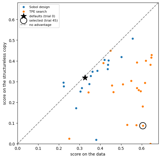
Scatter of the score on the data against the score on the structureless copy for each trial, with a dashed no-advantage line.

Each dot is one finished trial. The horizontal axis is its score on the data. The vertical axis is its score on the copy. The dashed diagonal marks equal scores, “no advantage”. Blue dots are the Sobol design and orange dots are TPE proposals. The star is the library defaults (trial 0) and the ring is the selected trial, here trial 45.

A dot on the diagonal gains nothing from the data. A dot far below it scores well on the data and poorly on the copy. The defaults sit on the diagonal, at about 0.33 on both axes. The selected trial sits at about 0.60 on the data and 0.09 on the copy.

The search’s own scores are optimistic, because the best of many noisy scores is partly luck (the winner’s curse). For the final choice, Starfold scores the top three and the defaults again on fresh subsets against fresh copies. This fresh re-score reduces the winner’s curse and does not remove it. Print the fresh gaps:

s = result.search
print(f"fresh gap over three fresh copies: selected {s.gap_selected:.3f}, defaults {s.gap_default:.3f}")

The recorded run prints:

fresh gap over three fresh copies: selected 0.372, defaults -0.001

The defaults gain nothing over the copy (a gap of -0.001) and the selected setting gains 0.372, so the search found a setting that uses structure the copy lacks. That comparison covers one setting on three copies and is not a test. The test comes next.

Step 10: read the calibration test result¶

The search picks the best of many settings, and the best of many settings scores well even on data with no groups. The calibration test asks how well that would look on structureless data. By default it replays trials 0 to 16 on each copy (the defaults and the 16-trial Sobol design, a set of settings spread evenly over the allowed ranges). Its statistic is the largest search gap among those 17 trials, not the best score of the full search. For this table the statistic is 0.362. The selected trial (trial 45) lies outside the 17, so 0.362 is not its gap. The test computes the same statistic on copies of the table and counts how many copies reach the table’s value. The p-value is (h + 1) / (L + 1), with L the copies run and h the copies at or above the table (Phipson and Smyth 2010, doi:10.2202/1544-6115.1585).

Each copy costs 102 fits. The test draws up to 19 copies (1,938 fits, about six times the fits of the rest of the run) and stops early once 3 copies reach the table’s value. Run it once, on the result you report, from the repository root:

python -m bench.null_stage apogee notebooks/runs/apogee --output output/null

The --output folder keeps your record apart from the recorded file bench/results/apogee_null.json, which the command would otherwise overwrite. Your record is output/null/apogee_null.json. The command does not change the saved result. To attach the test to the saved result and recompute its flags, add --update-result, which rewrites the files in notebooks/runs/apogee. The recorded run took 2,176 seconds (about 36 minutes) for 1,938 fits. From the recorded file:

quantity	value
table’s statistic (`exploration_design_max`)	0.362
copies run, copies at or above the table	19, 1
p-value	0.10
Monte Carlo interval on p	0.001 to 0.260
`structure_supported` (p at most alpha = 0.05)	false

One copy reached a best gap of 0.3655 against the table’s 0.3620. Since p is above 0.05, Starfold raises no_structure_supported once the test is attached to the result with --update-result. The test does not support structure at that level, for this family of copies.

Three reasons can explain that, and this run cannot separate them. The statistic uses only the 17 opening trials, and its power against the full-search statistic is not measured. With 19 copies, p moves in steps of 0.05, and one copy decided the outcome. The copy keeps a Gaussian dependence between iron, magnesium and the orbits, and that dependence may carry much of the two-sequence signal.

The Monte Carlo interval of 0.001 to 0.260 is wide because 19 copies are few. It is a 95 percent Clopper-Pearson interval (Clopper and Pearson 1934, doi:10.1093/biomet/26.4.404) for the chance that a copy reaches the table’s value. It says how well the simulation pinned the p-value, and not how sure you can be that the groups are real. The readings “p at most 0.05 means no copy reached the table” and “p above 0.05 means at least one did” hold at the default 19 copies only. See Calibration p-value. Report the groups as reproducible, and not as shown to exceed the copy.

Step 11: report it¶

The values of the recorded run (all stars, random_state=0, default budgets, laptop GPU):

quantity	value
groups, stars in each, unassigned	2 groups of 1,588 and 6,586 stars; 1,068 unassigned
groups per refit, 5 to 95 percent over 32 refits	2 to 2
group recurrence	0.91 (0.89 to 0.94) and 0.92 (0.88 to 0.94)
unresolved mass	0.154
co-association within, between, contrast	0.979, 0.003, 0.976
group medians of [Fe/H] and [Mg/Fe] (dex)	group 0: -0.42 and +0.27; group 1: -0.08 and +0.04
consensus agreement (the cut against the partition)	0.0, all 4,096 subset stars cut as noise
calibration p-value and interval	0.10 (0.001 to 0.260), 1 of 19 copies at or above

Name the evidence behind each number. The groups come from one fit of the selected setting on all stars. Recurrence, the count interval and the bands come from 32 refits on 80 percent subsets with new seeds. The p-value comes from the separate calibration run.

A wording that follows the evidence: “Starfold recovers 2 groups with recurrence 0.91 and 0.92 across 32 refits, whose medians lie on the high-alpha and low-alpha sequences. A matched Gaussian-copula test gives p = 0.10 (19 copies), so the split is not shown to exceed a single correlated population.” State the claim about the sequences only if the medians support it, as they do in step 7.

What the run does not support¶

It does not show that the groups are distinct populations. Reproducible is not true. At the default 19 copies, a p-value at or below 0.05 would say only that no copy scored as high as the table. A p-value above 0.05 says at least one did.
It does not show that the Milky Way holds this many populations. The count depends on the settings and on what you call a population. Its interval is over refits, not a confidence interval.
It gives no membership probability for any star. Support counts how often a star recurs with its group. HDBSCAN strengths describe one fit. Neither is a posterior.
It says nothing about the Galaxy as a whole. These are APOGEE stars with a signal-to-noise ratio above 70 and Gaia orbits inside a volume cut. No selection function (the chance that a star of a given kind enters the sample) was modelled.
It says nothing about measurement error. The table has no per-star uncertainties, so the bands reflect subsampling and seeds only.
It is not a citable result. The bundled table is for tutorials. For published work, rebuild it from APOGEE and Gaia using the provenance note in bench/data/stellar_chemokinematics_apogee_dr19.md.

What you learned¶

Two groups recur (0.91 and 0.92), the count interval is 2 to 2, and the unresolved mass is 0.154.
The co-association contrast is 0.976. The cut failed for a cause not diagnosed, which is a warning about the cut and says nothing against the groups.
The calibration test gave p = 0.10, so the split is reproducible and not shown to beat a structureless copy.

Look up a number on its own page:

Reproducibility: Group recurrence, Support and own support, Unresolved mass, Count interval.
Checks: Co-association, contrast and the consensus check, Calibration p-value.
Score terms: Score, Gap, Prediction agreement, Coverage, Modularity, Default comparison.
Group values: Group properties and their bands, HDBSCAN strengths.

Next page¶

To run the calibration test on your own result, see Run the calibration test. For the full list of how-to pages, see the How-to guides. To repeat the digits run, go back to Tutorial: groups in the scikit-learn digits dataset, part 1.